How Do You Know if Acceleration Is Constant From Time Vs Position Graph
Acceleration on a position vs. fourth dimension graph can be obtained, by having the initial position and velocity of a moving object.
In this article, we want to show you lot how to find constant acceleration from a position-fourth dimension graph with some solved bug.
Y'all can skip this introduction and refer to problems 6 and 7.
Types of Motion:
An object tin move at a constant speed or have a changing velocity.
Suppose you are driving a car at a constant speed of $100\,{\rm km/h}$ along a direct line. What does mean past $100\,{\rm km/h}$?
The speed of $100\,{\rm km/h}$ indicates that you drive the first 100 km in the offset 60 minutes, the next 100 km during the second hr, another 100 km for the third hour, and so on.
One time nosotros plot these successive equal displacements as a part of time, nosotros arrive at a straight line.
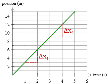
As you can encounter above, at equal fourth dimension intervals (here, 1 2nd) every second the displacements $\Delta x_1$ and $\Delta x_2$ are equal.
In such a type of movement, during each equal time interval, displacements are equal. This kind of motion is called uniform motion since, past definition of average dispatch, the object'southward acceleration is goose egg.
According to the definition of boilerplate velocity, $\bar{v}=\frac{10-x_0}{\Delta t}$, we can detect the position of a moving object at each instant by rearranging information technology every bit beneath \[10=vt+x_0\] This is a linear equation with a position vs. fourth dimension graph shown above.
Therefore, a motion in which equal displacements occur during any successive equal-time intervals is known every bit uniform movement.
Now, when the car has a changing velocity , and nosotros plot the positions of each betoken that the motorcar passes through information technology, nosotros make it at an arbitrary curve , in contrast to a direct line in the previous example.
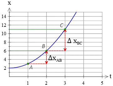
In the above, you can meet explicitly that at each equal time intervals (here, $ane\,{\rm s}$) the corresponding displacements are not equal i.e. $\Delta x_{BC}\ne \Delta x_{AB}$.
Therefore, the acceleration of such a move is not null.
In this case, the position of a moving object at any moment is given by the kinematics equation, $x=\frac 12 at^2 +v_0t+x_0$.
This equation tells the states that for an accelerated motility, position varies with time in a quadratic grade whose graph is shown above.
Overall, a constant velocity (compatible) motility has a directly line position-versus-time graph, but a curve in the $x-t$ graph represents an accelerated motion.
This curve for a constant acceleration has a simple grade of quadratic.
Direction of acceleration on a position-time graph
Acceleration is defined as avector quantity in physics with both a direction and a magnitude. We tin can discover both using a $x-t$ graph.
As mentioned in a higher place, the position of a uniform accelerating object varies with time as a quadratic function.
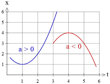
A positive acceleration ($a>0$) yields a position-time graph opening upward .
Similarly, a negative acceleration ($a<0$) produces a position-time graph opening downward . Both cases are shown in the effigy below
Magnitude of acceleration on a position-time graph
Information technology is a difficult task to notice the magnitude of the acceleration vector for a moving object from its position-fourth dimension graph.
If the object increases its speed at a abiding rate, then its acceleration is a constant value during that time interval.
In such cases, the position vs. time graph has a quadratic curve in which we can just observe its acceleration by having initial position and velocity.
In the post-obit, we will try to learn this calculation by a couple of solved examples.
Example (1): The equation of position vs. time for a moving object, in SI units, is equally $x=-t^2+6t-9$. Which of the following choices are correct?
(a) The object's acceleration is constant and its magnitude is $i\,{\rm m/s^2}$.
(b) The object's velocity at the initial time $t=0$ is to the negative $10$-axis.
(c) The object's initial position is on the negative side of the $x$-axis.
Solution: nosotros examine each option separately.
(a) This equation has a quadratic form so its acceleration is constant. Comparison this equation with standard constant acceleration kinematic equation, $x=\frac 12 at^2+v_0t+x_0$, we will find its magnitude as \[\frac 12 a=-ane \Rightarrow \ a=-2\,{\rm m/s^two}\] Then this choice is wrong.
(b) "Object's velocity at the initial time'' means its initial velocity. Comparison the two equations below reveals that initial velocity is $v_0=+6\,{\rm m/south}$.\brainstorm{gather*}10=\frac 12 at^2+v_0t+x_0 \\\\ ten=-t^ii+6t-9 \end{gather*} The positive sign indicates that the initial velocity is toward the positive $x$-axis. So, this choice is too incorrect.
(c) Past setting $t=0$ in the position-fourth dimension equation, its initial position is obtained. Then, $x_0=-ix\,{\rm m}$. Negative indicates that the object is on the negative side of the $x$-axis initially. Thus, this choice is correct.
Example (2): The position vs. time graph of a moving object accelerates uniformly forth the $x$ axis is plotted in the figure below. Discover its dispatch, initial velocity, and position.
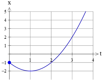
Solution: The concavity of the graph tells us nigh the sign of acceleration. Here, the graph opens upwards (concave upward), and then its dispatch is positive, $a>0$.
At the instant the motion is started $t=0$, the position of the object is a negative value. Information technology means that, initially, the object starts its motion on the negative side of the $ten$-axis.
Recall that the gradient of the position-time graph represents the object's velocity. A tangent line at time $t=0$ has a negative gradient because that makes an obtuse angle with the $+x$-centrality. So, the initial velocity is negative, as well.
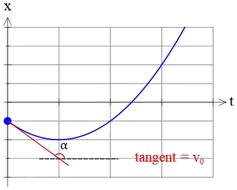
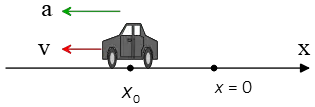
Overall, this object starts its motion at a position behind the origin in the opposite management of the $x$-axis as shown in the figure beneath.
In the next example, nosotros will discover the constant acceleration of a moving object using its position vs. time graph numerically.
Example (three): the position of a moving object (along a straight positive line) as a function of time is given by the curve shown in the figure beneath. Detect the acceleration of the object.
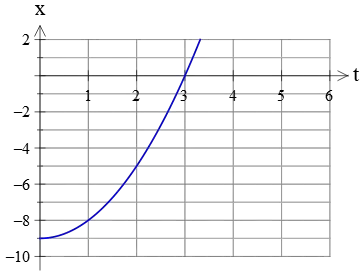
Solution: Get-go, collect all information that the plot gives us. At time $t=0$, the object is at position $x=-ix\,{\rm k}$ and at time $t=three\,{\rm s}$ its position is cypher, that is, it returns dorsum to its starting position.
The graph opens upward, indicating a positive acceleration.
It is said that the motion has a constant acceleration, and so its position versus time must be changed as a quadratic function which is adamant by the kinematics equation $x=\frac 12 at^ii+v_0t+x_0$.
In the in a higher place equation, $x_0$ is the position at time $t=0$ or the initial position. The graph shows united states that, for this object, it is $x_0=-9\,{\rm yard}$.
$v_0$ is also the initial velocity which is found by computing the gradient of the position-time graph at time $t=0$.
Every bit you can see, in this graph, the slope (in greenish) is parallel to the horizontal, makes an angle of zip, and consequently, its initial velocity is zip, $v_0=0$.
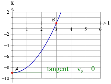
If we substitute these two finding into the standard kinematics equation $x=\frac 12 at^ii+v_0t+x_0$, we go \[x=\frac 12 at^ii-9\] The remaining quantity is the acceleration $a$.
In that location is some other signal that has non been used yet, $B=(x=0,t=3\,{\rm s})$. Substituting this point into the above equation, and solving for $a$ nosotros become \begin{align*} x&=\frac 12 at^2-9\\\\0&=\frac 12 (a)(3)^2-9\\\\\Rightarrow a&=2\quad {\rm m/s^2}\terminate{align*} Therefor, the object's acceleration is $ii\,{\rm grand/s^two}$.
Instance (4): A machine starts at rest and accelerates at a abiding rate in a direct line. Its position-versus-time graph is shown in the figure below. Find the car'south dispatch?
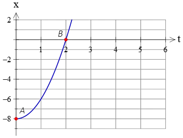
Solution: This is another example trouble that shows yous how to detect acceleration from a position vs. time graph.
Like previous example, locate two points on the graph with the given information. $A(10=-8\,{\rm k},t=0)$ and $B(x=0,t=2\,{\rm s})$. Using these two points and applying the kinematics equation $x=\frac 12 at^2+v_0t+x_0$, one can find the auto'southward acceleration.
Putting point $A$ into the higher up equation, gives united states \begin{align*} x&=\frac 12 at^2+v_0t+x_0\\\\-8&=\frac 12 a(0)^2+v_0(0)+x_0\\\\\Rightarrow \quad x_0&=-8\,{\rm m}\terminate{align*} It is said in the question that the car starts its motion from residue, then its initial velocity is nada, $v_0=0$. Now, substituting the second betoken $B$ into the standard equation, and solving for $a$, get \begin{align*}x&=\frac 12 at^2+v_0t+x_0\\\\0&=\frac 12 a(2)^2+0-8\\\\ 0&=2a-8\\\\\Rightarrow a&=4\quad {\rm one thousand/south^2}\end{marshal*} So with the assist of 2 points on the position vs. fourth dimension graph, we were able to find the acceleration of the object.
In the side by side instance, acceleration on a position-time graph gets in the case of having an initial velocity, $v_0\neq0$.
Example (6): The position vs. fourth dimension graph of a moving object along the positive $ten$-axis is equally follows. Find the object's dispatch.
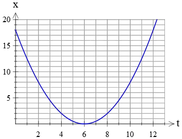
Solution: Equally ever, to detect the constant dispatch of a moving object from its position-versus-time graph, one should locate ii points on the graph and substitute them into the standard kinematics equation $10=\frac 12 at^two+v_0t+x_0$.
Here, initial betoken has coordinate $A(ten=eighteen\,{\rm grand},t=0)$ from which we tin detect the initial position, $x_0=xviii\,{\rm chiliad}$.
The other indicate is $B(x=0,t=6\,{\rm s})$. Given the initial position, substitute the point B into the standard kinematics equation, nosotros have \begin{assemble*} x=\frac 12 at^ii+v_0t+x_0\\\\0=\frac 12 a(half dozen)^2+v_0 (vi)+18 \\\\ \Rightarrow \boxed{18a+6v_0+18=0} \end{assemble*} As you can meet, we have one equation with 2 unknowns. We demand an boosted equation to exist able to notice the unknowns.
In the previous examples, the position-time graph had a cipher slope and thus become a aught initial velocity.
Of the graph, we see that the slope at fourth dimension $t=0$ is not cypher then the object does not starting time from residual.
But how to notice another equation?
To find that equation, we pay attention to an of import notation below:
The tangent line at betoken $B$ is horizontal and then velocity at that time is cypher, according to the equivalence of gradient and velocity on a $x-t$ graph.
Substituting this extra information into another kinematics equation, $v=v_0+at$, we can find the initial velocity. \begin{get together*} v=v_0+at\\0=v_0+a(6)\\ \Rightarrow \boxed{6a+v_0=0} \finish{gather*} Solving the above equation for $v_0$, we go $v_0=-6a$.
Now, substitute it into the beginning equation $18a+6v_0+18=0$ and solve for the unknown acceleration \begin{gather*} 18a+6v_0+18=0\\ 18a+half-dozen(-6a)+eighteen=0\\ \Rightarrow a=1\quad {\rm one thousand/s^2}\terminate{gather*} If nosotros put this value into $v_0=-6a$, the initial velocity is also found.
Consequently, the machine starts its motion toward the negative $ten$ axis with an initial velocity of vi m/s and increases its speed at a abiding rate of $1\,{\rm grand/s^2}$.
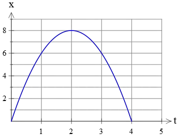
Case (vii): The position vs. time graph of a moving object forth a direct line is a parabola equally below. Detect the equation of the object's velocity as a part of time?
Solution:
Physical interpretation of graph: This object starts its movement at some initial velocity (because the slope at time $t=0$ makes an angle with horizontal) and decreases its speed at a constant charge per unit (i.e. $a<0$ as tin can be seen from the concavity downwards of the curve) until reaches point B where its velocity gets zero, changes its direction, and returns to the starting point in the contrary direction.
As you lot guess, this is exactly a description for motion that appears in a gratis-fall. In add-on, such a graph appears too in the projectile move problems.
Equally said, the curve of the position-time graph is a parabola that has a quadratic course. So, the object has a constant acceleration.
On the other side, the curve opens downward, so the acceleration is negative $a<0$.
In this curve, the coordinate of iii points are given, $A(x=0,t=0)$, $B(ten=8\,{\rm m},t=2\,{\rm s})$, and $C(x=0\,{\rm 1000}, t=four\,{\rm s})$.
The velocity of an object with a constant acceleration changes with time as $five=v_0+at$. Thus, we must detect its initial velocity too as dispatch.
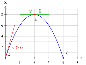
To find the unknowns, it is meliorate to apply kinematics equations between any two given points. Between points A and B, displacement is computed as \[\Delta 10=x_B-x_A=eight-0=8\quad{\rm k}\] Using kinematics equation, $v^two-v_0^2=2a\Delta x$, for these two points, we have \begin{gather*} v_B^two-v_A^2=2a\Delta 10\\\\0-v_0^ii=ii(a)(8)\\\\\Rightarrow\quad \boxed{v_0^2=-16a}\stop{gather*} where we used this note that velocity at indicate B is nada because the slope of the tangent line at that signal is horizontal.
At present, we cull points A and C, compute their displacement, and apply the kinematics equation $x-x_0=\frac 12 at^2+v_0t$ \[\Delta 10=x_C-x_A=0-0=0\] As expected since the objects returns to its starting indicate. \brainstorm{assemble*} \Delta 10=\frac 12 at^2+v_0t\\\\0=\frac 12 (a)(four)^2+v_0(4)\\\\ \Rightarrow \quad \boxed{8a+4v_0=0} \end{gather*} Until now, we take 2 equations with two unknowns which is completely solvable.
The second equation, $8a+4v_0=0$, gives usa $v_0=-2a$. Now, substitute information technology into the first equation \begin{gather*} v_0^2=-16a\\\\ (-2a)^two=-16a\\\\4a^2=-16a\\\\ \rightarrow\quad 4a(a+4)=0\end{assemble*} Solving this equation for $a$, we become two solutions $a=0$, and $a=-iv\,{\rm m/southward^ii}$.
The zilch acceleration $a=0$ is not plausible, since it represents a constant velocity move whose position-time graph is a straight line but in this problem, we take a curve.
Therefore, the acceptable acceleration is $a=-4\,{\rm m/south^two}$. By substituting this into either get-go ($v_0^2=-16a$) or second equation ($8a+4v_0$), and solving for $v_0$, we will get the initial velocity, \brainstorm{assemble*} 8a+4v_0=0 \\ \rightarrow (8)(-4)+4v_0=0\\ \Rightarrow v_0=viii\,{\rm m/s}\end{get together*} Every bit expected, since the tangent line at time $t=0$ has a positive slope.
Substituting these known values into the kinematics equation $v=v_0+at$, we will obtain the object's velocity as a function of time. \[v=eight-4t\] This equation gives the variation of velocity as a function of time. When this equation is plotted, a velocity-time graph is obtained.
Summary:
In this article, we found out how to compute the object's abiding acceleration using a position-time graph.
Having the initial velocity $v_0$, calculate the displacement $\Delta x$ betwixt ii known points on the graph. Next, use the kinematics equation $\Delta x=\frac 12 at^2+v_0t$ and solve for the unknown acceleration $a$.
If the object has an initial velocity, and then we demand at least three points on the graph with known position and time coordinates.
In this example, the kinematics equation $v^2-v_0^2=2a\Delta x$ is also used.
Author: Dr. Ali Nemati
Page Published: 8-xiii-2021
andersonhonsintepher00.blogspot.com
Source: https://physexams.com/blog/acceleration-on-position-time-graph_17
0 Response to "How Do You Know if Acceleration Is Constant From Time Vs Position Graph"
Post a Comment